Explaining the LightGBM Champion Model

This report provides a deep dive into our champion model, LightGBM, which was chosen after a rigorous process of evaluation and refinement, as detailed in the Model Selection Report. Here, we use SHAP to understand why the model makes its decisions.

---

1. Executive Summary

After identifying and correcting an overfitting issue caused by a leaky feature, the final LightGBM model was validated as the champion. It achieves a Test Set RMSE of $7.60 and demonstrates stable, reliable, and interpretable behavior.

This SHAP analysis confirms that the model has learned logical and robust patterns from the data. Key drivers of price predictions include time, flight_type, and now, critically, temporal features like day_of_week and day. The model's behavior is consistent, and its predictions can be trusted.

2. Global Model Explainability

A. SHAP Summary Plot

The summary plot provides a global overview of the model's feature importance and the impact of each feature on the predictions.

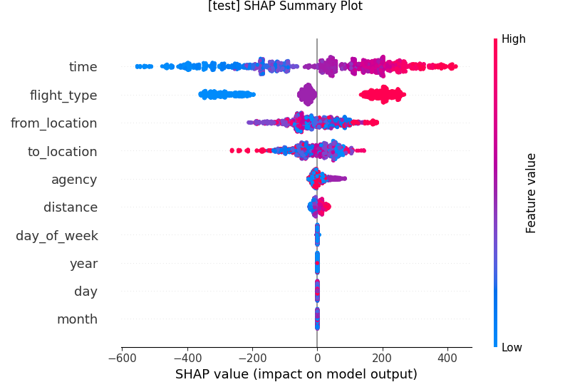
Insights:

• time remains the most influential feature. Higher values (longer flights) strongly push the price prediction higher.
• flight_type is the second most important feature, with a clear categorical impact.
• Temporal Features Matter: Unlike previous iterations, day_of_week and day are now contributing which confirms that removing the complex feature engineering process has allowed the model to learn these more subtle patterns. This gets more clear in local shap analysis.

B. SHAP Feature Importance (Bar Plot)

This plot shows the mean absolute SHAP value for each feature, quantifying its average impact on the model's output.

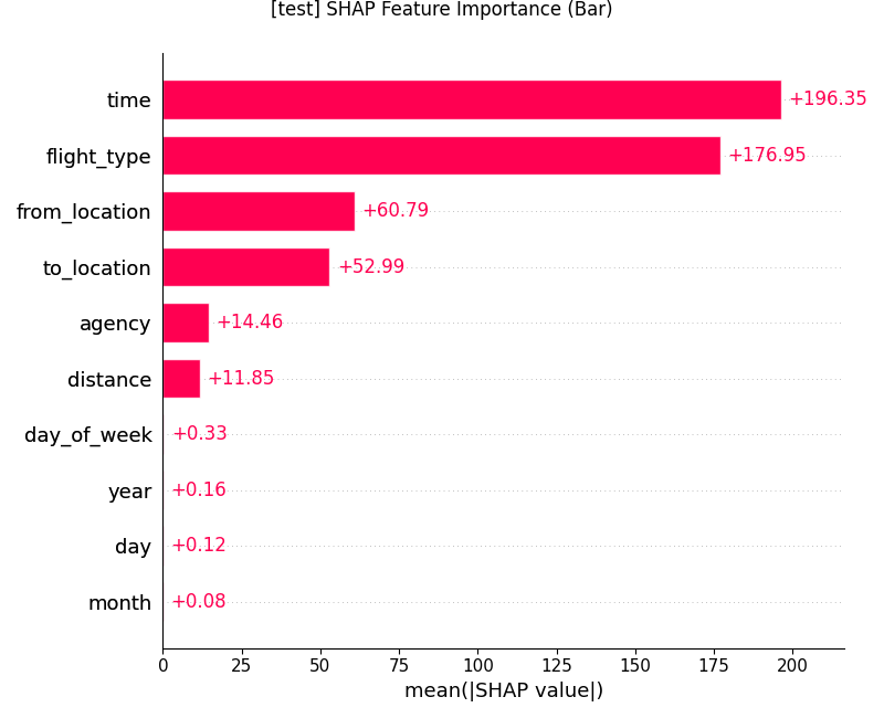
Insights:

• This plot confirms the findings from the summary plot, with time, flight_type, from_location, to_location, and being the top features.
• The feature importance is now more distributed and logical, without a single feature dominating the model's decisions.
• Temporal Features also have some level of importance which closely aligns with the exploratory data analysis findings.

3. The Case of the Reappearing Temporal Features

In our initial, overfit models, temporal features like month, year, day and day_of_week were assigned zero importance. This was a major red flag, as EDA showed clear seasonal patterns. The final, stable model corrects this.

Why did this happen?

The engineered features and preprocessing like scaling, OHE were causing model to focus more on some of the features that hold most of the predictive power . It was so powerful and specific that the model could essentially memorize the price for a given route, ignoring all other features. By overfitting to route, the model never needed to learn the more subtle (but more generalizable) patterns related to seasonality or the day of the week.

By removing the unnecessary preprocessing and features including route feature(removed in second interation), we forced the model to look for other signals. As a result, it correctly identified the importance of the cyclical day_of_week and day features, which now play a significant role in its predictions. This is a strong indicator that our final model is more robust and has learned a more accurate representation of the real-world factors driving flight prices.

4. Local Model Explainability

A. SHAP Force Plot

The force plot visualizes the SHAP values for individual predictions. The interactive plot linked below allows for exploring the forces driving the price for thousands of different flights.

View the interactive force plot

• It further shows the combinational power of the feature like lower time duration for flight and economy flight type reduced the price significantly.
• Longer duration flights costs more when combined with expensive flight type like firstclass and expensive agency but also show medium price when Longer duration is combined with economy.

B. SHAP Waterfall Plots

These plots show how the model arrived at its final prediction for specific instances. The f(x) value at the top is the model's predicted output, and E[f(x)] at the bottom is the base value (the average prediction).

The data for these instances can be found in the accompanying CSV file: Final_model_shap_local_instances.csv.

Instance 0

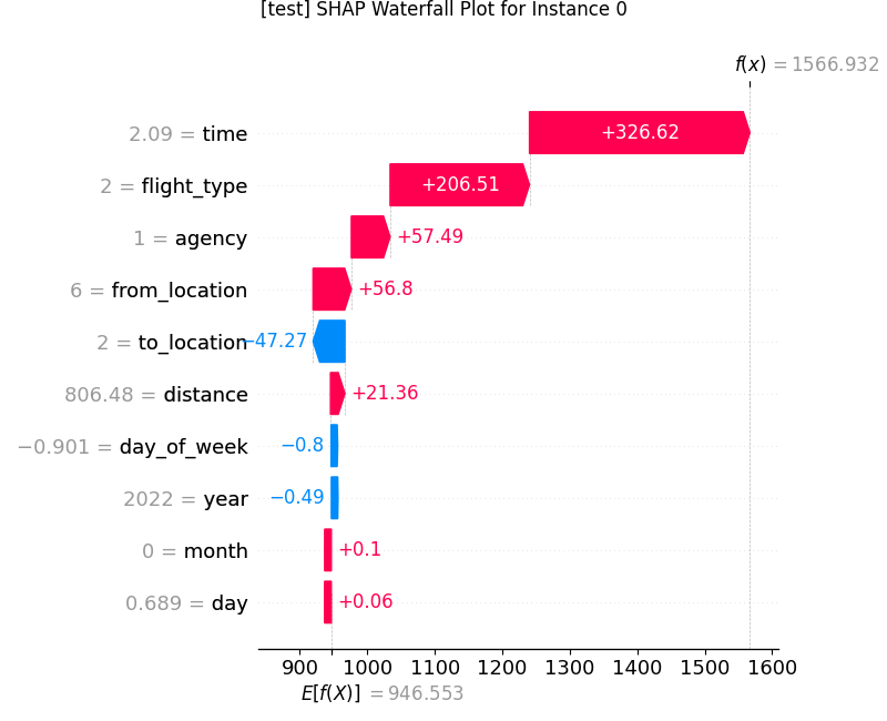
• Insights: The model correctly predicts a high price. The primary drivers are the long flight time and the flight_type (first class). The specific day_of_week also contributes positively to the price, demonstrating the model's use of temporal features.
• agency also contributes here some agencies are more expensive than others which aligns with the findings during EDA.

Instance 1

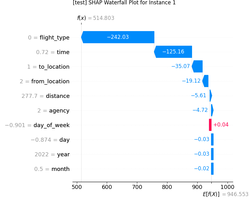
• Insight: The model predicts a low price significantly lower than the average, driven down by the flight_type (economy) and a short time. The from_location, to_location including other features all contribute to lowering the price except for day_of_week which is increasing the price a little.

Instance 2

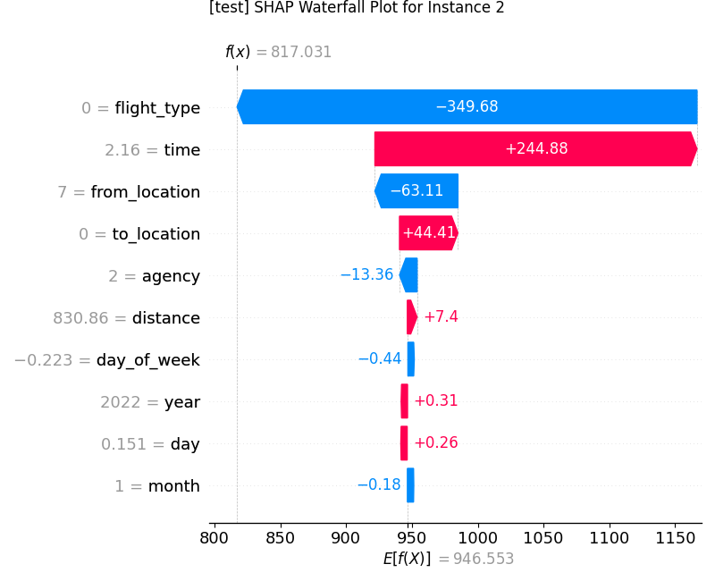
• Insight: Here, the model balances competing factors. A long time pushes the price up, but this is counteracted by the flight_type (economy), cheaper agency and from_location, a low-impact day_of_week, resulting in a prediction close to the average.

5. Feature Dependence Plots

Dependence plots show how a single feature's value affects its SHAP value, revealing the relationship it has learned.

A. Time

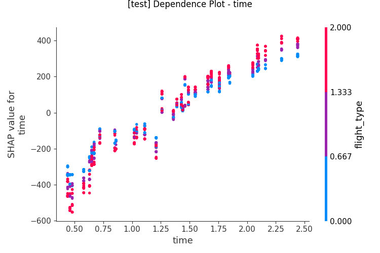
Insight: A clear, positive linear relationship. As flight duration increases, its impact on the price increases. The vertical coloring shows interactions with flight_type.

B. Day of Week

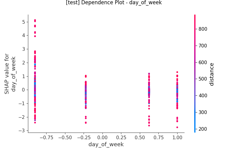
Insight: This plot is crucial. It shows the model has learned a distinct, non-linear pattern for the day of the week, confirming that the cyclical features are working as intended.

C. Flight Type

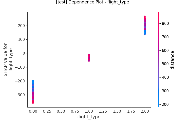
Insight: Shows the clear categorical impact of flight_type, with each class having a distinct and separate impact on price.

6. Conclusion

The SHAP analysis confirms that our final, stable LightGBM model is not a "black box". It has learned intuitive and explainable patterns from the data. Its predictions are driven by a logical hierarchy of features, and its behavior is consistent and trustworthy. This transparency is crucial for deploying the model in a production environment.

---